Neo4j Graph Hack 2016: Where to avoid cycling accidents
It’s a little late but it’s taken me a while to finally get this blog up and running; Now that it is live I’m catching up publishing interesting projects from the past. I’ve been intrigued by graph databases since I discovered them and curious about what they are capable of (another example can be seen in this blog post). So having won a ticket to the Graph Connect Europe 2016 conference I thought I’d take advantage of attending the graph hack hosted by Neo Technologies the night before. I also invited a friend, Amy, along. Together we formed Crash Dodgers (follow the link to get the actual Python notebook) and decided to see if we could find the most dangerous spots to hire bicycles in London, in the 2-3 hours we had available to us!
**tldr: We won the “best app” award **
Graph hack 2016 @ GraphConnect Europe
Using Neo4j with transport data
Team: Crash Dodgers: Adam Hill & Amy McQuillan
Concept: Combine Santander Bike data with cyclist accident data to find dangerous places to hire bikes in London
First up lets find all the Santander bike stations in London:
- Cycle hire updates with all stations are available from the TfL API here: link
- To make my life easier used http://codebeautify.org/xmltojson to convert to JSON and save the file locally
import pandas as pd
import numpy as np
import json
stations = json.load(open('./GraphHackData/bikeStation.json', 'r'))
stationsDF = pd.DataFrame(stations['stations']['station'])
stationsDF.tail()
| id | installDate | installed | lat | locked | long | name | nbBikes | nbDocks | nbEmptyDocks | removalDate | temporary | terminalName | |
|---|---|---|---|---|---|---|---|---|---|---|---|---|---|
| 754 | 794 | 1456404240000 | true | 51.474567 | false | -0.12458 | Lansdowne Way Bus Garage, Stockwell | 15 | 28 | 13 | false | 300204 | |
| 755 | 795 | 1456744740000 | true | 51.527566 | false | -0.13484927 | Melton Street, Euston | 5 | 28 | 23 | false | 300203 | |
| 756 | 800 | 1457107140000 | true | 51.4811219398 | false | -0.149035374873 | Sopwith Way, Battersea Park | 23 | 30 | 7 | false | 300248 | |
| 757 | 801 | true | 51.5052241745 | false | -0.0980318118664 | Lavington Street, Bankside | 26 | 29 | 3 | false | 300208 | ||
| 758 | 804 | true | 51.5346677396 | false | -0.125078652873 | Good's Way, King's Cross | 17 | 27 | 10 | false | 300243 |
Let’s store these stations as the first nodes of our graph
from py2neo import Graph
from py2neo import Node, Relationship
graph = Graph("http://neo4j:password@localhost:7474/db/data")
#Loop over all bike stations and store their details in Neo4j
for r, data in stationsDF.iterrows():
    tempNode = Node("Bike_station", a_Id = np.int(data['id']))
    tempNode['latitude'] = np.float(data.lat)
    tempNode['longitude'] = np.float(data.long)
    tempNode['name'] = data['name']
    tempNode['installDate'] = data.installDate
    tempNode['num_docks'] = np.int(data.nbDocks)
    graph.create(tempNode)
Traffic accidents in the UK
We look at data from 2014 regarding traffic accidents across the UK from here https://data.gov.uk/dataset/road-accidents-safety-data . We used the following files:
- 2014 Road Safety - Accidents 2014
- 2014 Road Safety - Vehicles 2014
- 2014 Road Safety - Casualties 2014
- Lookup up tables for variables
Local copies were downloaded and stored in ./GraphHackData
accidents = pd.read_csv('./GraphHackData/DfTRoadSafety_Accidents_2014.csv')
vehicles = pd.read_csv('./GraphHackData/DfTRoadSafety_Vehicles_2014.csv')
casualties = pd.read_csv('./GraphHackData/DfTRoadSafety_Casualties_2014.csv')
Some strange characters are in some of the column names so let’s strip them out and then then merge accidents and casualties on Accident_Index
accidents = accidents.rename(columns={'Accident_Index': 'Accidents_Index'})
vehicles = vehicles.rename(columns={'Accident_Index': 'Accidents_Index'})
casualties = casualties.rename(columns={'Accident_Index': 'Accidents_Index'})
accidentsDF = pd.merge(accidents, casualties, on='Accidents_Index')
accidentsDF.head()
| Accidents_Index | Location_Easting_OSGR | Location_Northing_OSGR | Longitude | Latitude | Police_Force | Accident_Severity | Number_of_Vehicles | Number_of_Casualties | Date | ... | Age_of_Casualty | Age_Band_of_Casualty | Casualty_Severity | Pedestrian_Location | Pedestrian_Movement | Car_Passenger | Bus_or_Coach_Passenger | Pedestrian_Road_Maintenance_Worker | Casualty_Type | Casualty_Home_Area_Type | |
|---|---|---|---|---|---|---|---|---|---|---|---|---|---|---|---|---|---|---|---|---|---|
| 0 | 201401BS70001 | 524600 | 179020 | -0.206443 | 51.496345 | 1 | 3 | 2 | 1 | 09/01/2014 | ... | 49 | 8 | 3 | 0 | 0 | 0 | 0 | 0 | 8 | 1 |
| 1 | 201401BS70002 | 525780 | 178290 | -0.189713 | 51.489523 | 1 | 3 | 2 | 1 | 20/01/2014 | ... | 27 | 6 | 3 | 0 | 0 | 0 | 0 | 0 | 1 | -1 |
| 2 | 201401BS70003 | 526880 | 178430 | -0.173827 | 51.490536 | 1 | 3 | 2 | 1 | 21/01/2014 | ... | 27 | 6 | 3 | 0 | 0 | 0 | 0 | 0 | 3 | 1 |
| 3 | 201401BS70004 | 525580 | 179080 | -0.192311 | 51.496668 | 1 | 3 | 1 | 1 | 15/01/2014 | ... | 31 | 6 | 3 | 1 | 1 | 0 | 0 | 2 | 0 | 1 |
| 4 | 201401BS70006 | 527040 | 179030 | -0.171308 | 51.495892 | 1 | 3 | 2 | 1 | 09/01/2014 | ... | 32 | 6 | 3 | 0 | 0 | 0 | 0 | 0 | 9 | 1 |
5 rows × 46 columns
Which accidents are in London?
Santander bikes are only available in London so we also need to be able to filter by whether an accident is in London. Accidents are all assigned to LSOA (Lower Layer Super Output Area).
We identify all the LSOAs in London using this ref: http://data.london.gov.uk/dataset/lsoa-atlas
london = pd.read_excel('./GraphHackData/lsoa-data.xls', sheet='iadatasheet1', skiprows=2)
lsoa = set(london.Codes)
#Add a boolean column to the accidents dataframe to describe if in London
accidentsDF['in_London'] = accidentsDF.LSOA_of_Accident_Location.map(lambda x: x in lsoa)
From the DoT lookup table we identify that any casualty listed as 1 is a cyclist and hence we can now find all accidents in London in 2014 where the casualty was a cyclist
cyclingAccidents = accidentsDF[(accidentsDF['in_London'] == True) & (accidentsDF.Casualty_Type == 1)]
#Example incident
example = cyclingAccidents.loc[59,]
example
Accidents_Index                                201401BS70065
Location_Easting_OSGR                                 526610
Location_Northing_OSGR                                177280
Longitude                                          -0.178126
Latitude                                             51.4803
Police_Force                                               1
Accident_Severity                                          3
Number_of_Vehicles                                         2
Number_of_Casualties                                       1
Date                                              08/02/2014
Day_of_Week                                                7
Time                                                   18:20
Local_Authority_(District)                                12
Local_Authority_(Highway)                          E09000020
1st_Road_Class                                             3
1st_Road_Number                                         3220
Road_Type                                                  6
Speed_limit                                               30
Junction_Detail                                            0
Junction_Control                                          -1
2nd_Road_Class                                            -1
2nd_Road_Number                                            0
Pedestrian_Crossing-Human_Control                          0
Pedestrian_Crossing-Physical_Facilities                    5
Light_Conditions                                           4
Weather_Conditions                                         2
Road_Surface_Conditions                                    2
Special_Conditions_at_Site                                 0
Carriageway_Hazards                                        0
Urban_or_Rural_Area                                        1
Did_Police_Officer_Attend_Scene_of_Accident                2
LSOA_of_Accident_Location                          E01002840
Vehicle_Reference                                          2
Casualty_Reference                                         1
Casualty_Class                                             1
Sex_of_Casualty                                            1
Age_of_Casualty                                           32
Age_Band_of_Casualty                                       6
Casualty_Severity                                          3
Pedestrian_Location                                        0
Pedestrian_Movement                                        0
Car_Passenger                                              0
Bus_or_Coach_Passenger                                     0
Pedestrian_Road_Maintenance_Worker                         0
Casualty_Type                                              1
Casualty_Home_Area_Type                                   -1
in_London                                               True
Name: 59, dtype: object
Let’s see what the two nearest Santander bike stations are to this accident …
query = "MATCH (b:Bike_station) WITH b, distance(point(b), point({{latitude:{0}, longitude:{1}}})) AS dist RETURN b.a_Id AS station_id, b.name AS station_name, dist ORDER BY dist LIMIT 2".format(example.Latitude, example.Longitude)
cypher = graph.cypher
result = cypher.execute(query)
result
   | station_id | station_name                    | dist
---+------------+---------------------------------+-------------------
 1 |        746 | Lots Road, West Chelsea         | 99.27002411121134
 2 |        649 | World's End Place, West Chelsea |  227.456404989975
** So first piece of insight appears to be not to cycle at “World’s End”! **
Before generating the graph of the accidents we need to convert many of the numerical classifications into their human readable form to make things easier to interpret
#Conversion for some of the accident variables to huamn readable form

roadClass = {1: "Motorway",
             2: "A(M)",
             3: "A",
             4: "B",
             5: "C",
             6: "Unclassified"}

dow = {1: "Sunday",
       2: "Monday",
       3: "Tuesday",
       4: "Wednesday",
       5: "Thursday",
       6: "Friday",
       7: "Saturday"}

lightConditions = {1: "Daylight",
                   4: "Darkness: lights lit",
                   5: "Darkness: lights unlit",
                   6: "Darkness: no lighting",
                   7: "Darkness: lighting unknown",
                   -1: "Data missing"}

weatherConditions = {1:"Fine no high winds",
                     2:"Raining no high winds",
                     3:"Snowing no high winds",
                     4:"Fine + high winds",
                     5:"Raining + high winds",
                     6:"Snowing + high winds",
                     7:"Fog or mist",
                     8:"Other",
                     9:"Unknown",
                     -1:"Data missing"}

roadConditions = {1: "Dry",
                  2: "Wet or damp",
                  3: "Snow",
                  4: "Frost or ice",
                  5: "Flood over 3cm deep",
                  6: "Oil or diesel",
                  7: "Mud",
                 -1: "Data missing"}

gender = {1: "Male",
          2: "Female",
          3: "Not known",
          -1: "Data missing"}

severity ={1: "Fatal",
           2: "Serious",
           3: "Slight"}
Now we are ready to generate accident nodes and map them to the two nearest bike stations ** N.B. we will not map if the nearest bike station isn’t within 2km of an accident as Santander bike stations are concentrated in the centre rather than across the whole of what is labelled London **
def genAccidentNodes(datum):
    """For a given row in the accidents dataframe construct the appropriate set of nodes and relationships"""
    accident = Node("Accident", a_Id = datum.Accidents_Index)
    accident['latitude'] = datum.Latitude
    accident['longitude'] = datum.Longitude
    accident['severity'] = severity[datum.Casualty_Severity]
    accident['severity_score'] = 4. - datum.Casualty_Severity
    accident['time'] = datum.Time
    graph.create(accident)
    date = graph.merge_one('Date', "value", datum.Date)
    date.properties['day_of_week'] = dow[datum.Day_of_Week]
    graph.push(date)
    rel_1 = Relationship(accident, "HAPPENED_ON", date)

    #Make vector of relationships to create
    relationships = []
    relationships.append(rel_1)

    weatherCon = weatherConditions.get(datum.Weather_Conditions, "Data missing")
    if weatherCon != "Data missing":
        weather = graph.merge_one('Weather', "condition", weatherCon)
        relationships.append(Relationship(accident, "WITH", weather))
    lightCon = lightConditions.get(datum.Light_Conditions, "Data missing")
    if lightCon != "Data missing":
        light = graph.merge_one('Light', "condition", lightCon)
        relationships.append(Relationship(accident, "WITH", light))
    roadSurfaceCon = roadConditions.get(datum.Road_Surface_Conditions, "Data missing")
    if roadSurfaceCon != "Data missing":
        roadSurf = graph.merge_one('Road_surface', "condition", roadSurfaceCon)
        relationships.append(Relationship(accident, "WITH", roadSurf))

    speed = graph.merge_one("Speed_limit", "value", np.int(datum.Speed_limit))
    relationships.append(Relationship(accident, "WITH", speed))

    #And find the nearest bike stations
    query = "MATCH (b:Bike_station) WITH b, distance(point(b), point({{latitude:{0}, longitude:{1}}})) AS dist RETURN b.a_Id AS station, dist ORDER BY dist LIMIT 2".format(datum.Latitude, datum.Longitude)
    result = cypher.execute(query)
    #Only do this for bike sations where the nearest station is less than 2km away
    if result.records[0].dist <= 2000.:
        for i,rec in enumerate(result.records):
            bikeStation = graph.merge_one("Bike_station", "a_Id", rec.station)
            tempRel = Relationship(accident, "CLOSE_TO", bikeStation, distance=round(rec.dist,2), proximity=i+1)
            relationships.append(tempRel)

    graph.create(*relationships)
Let’s run the function over all London cycling accidents
output = cyclingAccidents.apply(genAccidentNodes, axis=1)
Graphically exploring our new database
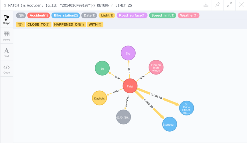
An accident node and associated properties including closest bike docking stations
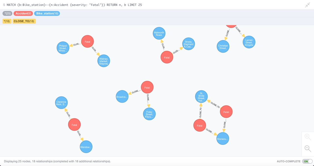
Which bike docking stations are linked to the fatal cycling accidents?
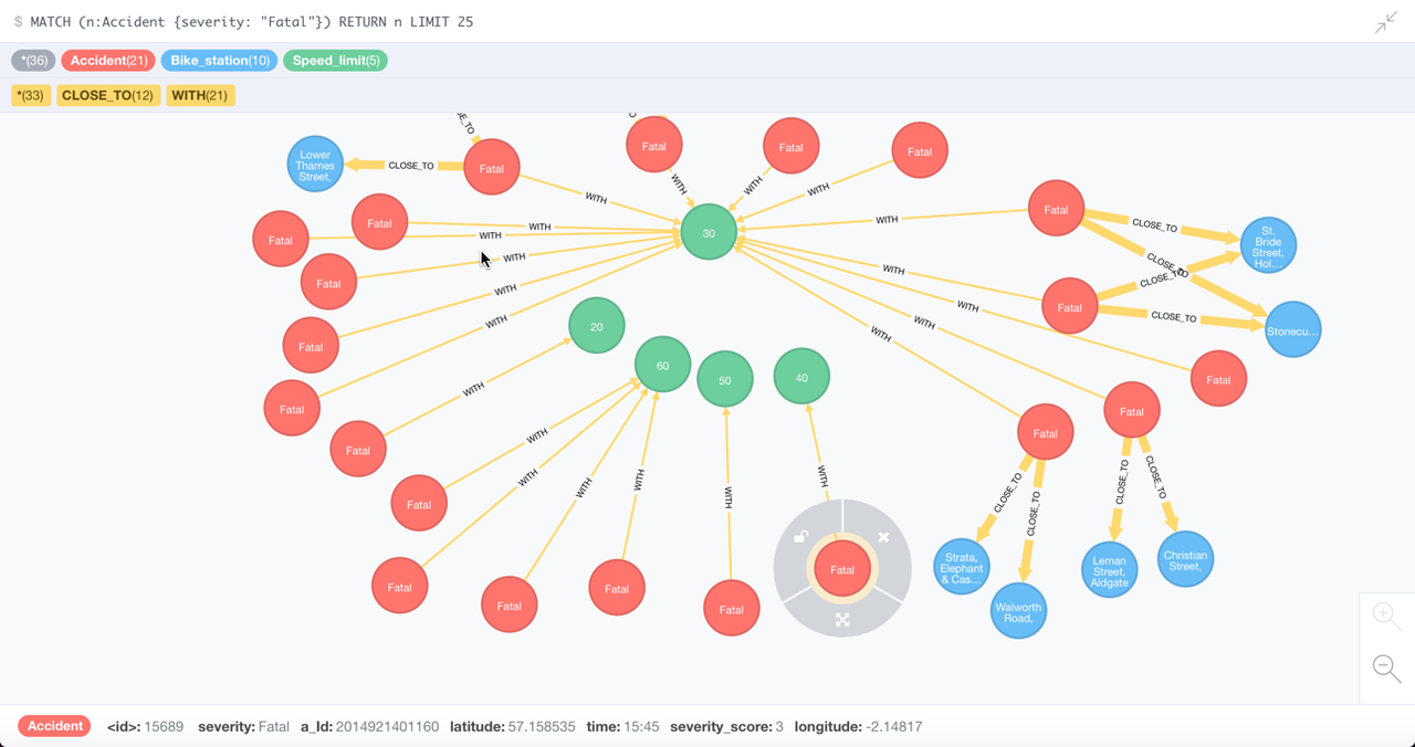
What was the speed limit on the roads with fatal cycling accidents?
The most dangerous bike docking stations to cycle between
We can query neo4j to count the number of accidents between bike stations
query = """MATCH (b1:Bike_station)<-[:CLOSE_TO]-(a:Accident)-[:CLOSE_TO]->(b2:Bike_station)
WITH b1, b2, COLLECT(DISTINCT a.a_Id) AS accidents
WHERE b1.a_Id < b2.a_Id
RETURN b1.name AS station1, b1.longitude AS lon1, b1.latitude AS lat1,
       b2.name AS station2, b2.longitude AS lon2, b2.latitude AS lat2,
       size(accidents) AS num_accidents
ORDER BY num_accidents DESC;"""
result = cypher.execute(query)
The top 10 most dangerous bike station pairs are …
df = pd.DataFrame(result.records, columns=result.columns)
df.head(10)
| station1 | lon1 | lat1 | station2 | lon2 | lat2 | num_accidents | |
|---|---|---|---|---|---|---|---|
| 0 | Clarence Walk, Stockwell | -0.126994 | 51.470733 | Binfield Road, Stockwell | -0.122832 | 51.472510 | 61 |
| 1 | Shoreditch Court, Haggerston | -0.070329 | 51.539084 | Haggerston Road, Haggerston | -0.074285 | 51.539329 | 48 |
| 2 | Islington Green, Angel | -0.102758 | 51.536384 | Charlotte Terrace, Angel | -0.112721 | 51.536392 | 32 |
| 3 | Ravenscourt Park Station, Hammersmith | -0.236770 | 51.494224 | Hammersmith Town Hall, Hammersmith | -0.234094 | 51.492637 | 32 |
| 4 | Bricklayers Arms, Borough | -0.085814 | 51.495061 | Rodney Road , Walworth | -0.090221 | 51.491485 | 30 |
| 5 | Napier Avenue, Millwall | -0.021582 | 51.487679 | Spindrift Avenue, Millwall | -0.018716 | 51.491090 | 28 |
| 6 | Ada Street, Hackney Central | -0.060292 | 51.535717 | Victoria Park Road, Hackney Central | -0.054162 | 51.536425 | 26 |
| 7 | Wandsworth Rd, Isley Court, Wandsworth Road | -0.141813 | 51.469260 | Heath Road, Battersea | -0.146545 | 51.468669 | 24 |
| 8 | Caldwell Street, Stockwell | -0.116493 | 51.477839 | Binfield Road, Stockwell | -0.122832 | 51.472510 | 23 |
| 9 | Stebondale Street, Cubitt Town | -0.009205 | 51.489096 | Saunders Ness Road, Cubitt Town | -0.009001 | 51.487129 | 23 |
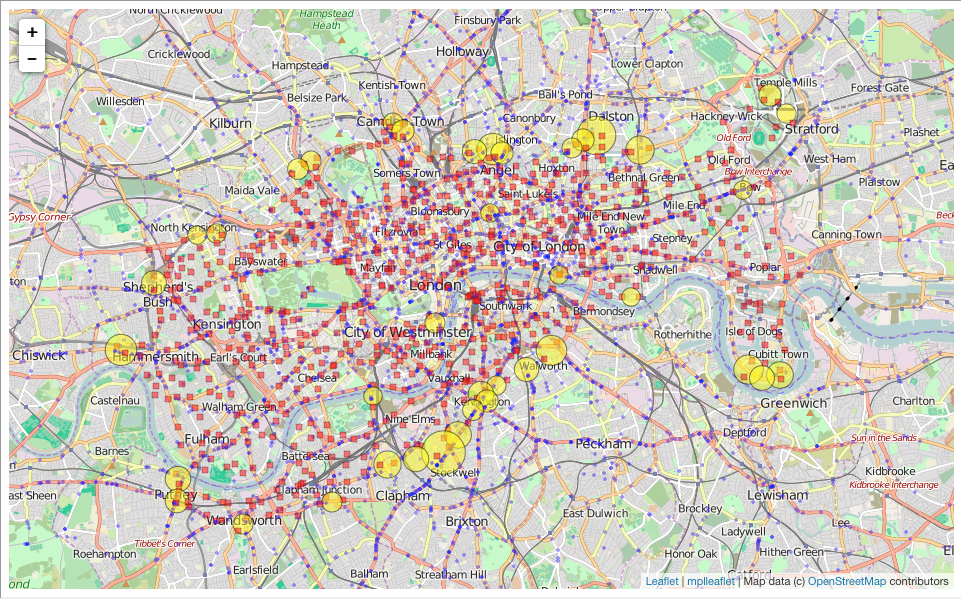
Plotting everything out looks like this
df['mean_longitude'] = (df.lon1+df.lon2)/2.
df['mean_latitude'] = (df.lat1+df.lat2)/2.
df2 = df[df.num_accidents > 10]
%matplotlib inline
import geopandas as gpd
import matplotlib.pyplot as plt
import mplleaflet

plt.rcParams['figure.figsize'] = 14, 10
fig = plt.figure()
plt.plot(cyclingAccidents.Longitude, cyclingAccidents.Latitude, 'b.', alpha=0.4, label='cycling accidents (2014)')
plt.plot(stationsDF.long, stationsDF.lat, 'rs', alpha=0.5, label='docking stations')
plt.scatter(df2.mean_longitude, df2.mean_latitude, s=df2.num_accidents*25, c='yellow', alpha=0.5, label='Most accidents')
plt.xlim(-0.25, 0.)
plt.ylim(51.45, 51.55)
#plt.legend(loc='lower right')
(51.45, 51.55)
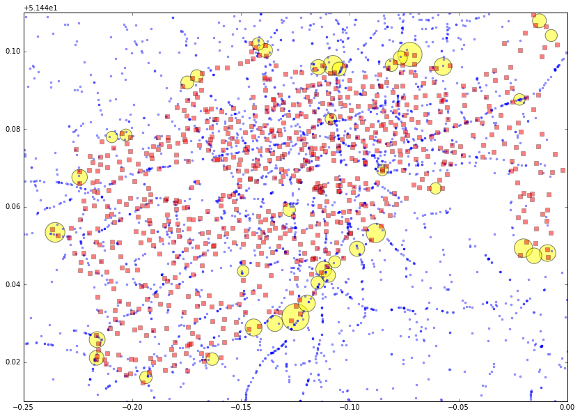
Can combine this with a map to get a better feel for where in London we are
mplleaflet.display(fig=fig, tiles='osm')

Conclusions
Some interesting first results but more work needed
It’s great to see that the initial analysis worked and using Neo4j made our analysis easier and there is a lot more data stored in there that could be analysed at a later date. What at first appears surprising is that the “danger stations” that we have identified appear to gnerally bound the region that Santander bikes are available in, however, we cannot confirm these are correct without correcting for a couple of additional observational biases:
- Normalise for the amount of journeys starting/ending at each station, i.e. do more accidents happen because more people are riding in these parts of London.
- The density of bike docking stations is not uniform so those on the periphery may be being assigned more accidents based upon fewer stations to assign the accidents to.
Enjoyed this post?
Share it with your colleagues, network, or friends: